Using an AI Agent to explore game dynamics in 1010!
Intro
For a while now I’ve been interested in AI accelerated design space exploration. It’s a compelling approach that allows the rapid iteration of game rules and balance. As someone who’s spent a lot of their career working on early stage prototypes, I’ve seen firsthand how important it is to nail the core mechanics of a game.
So how does that work? You first need to train an agent that is capable of playing the game in a way that it can react to balance changes and even rule changes. Then you define some metrics based on game dynamics that I’ll cover in the next section, before changing the game balance and rules to hit those metrics.

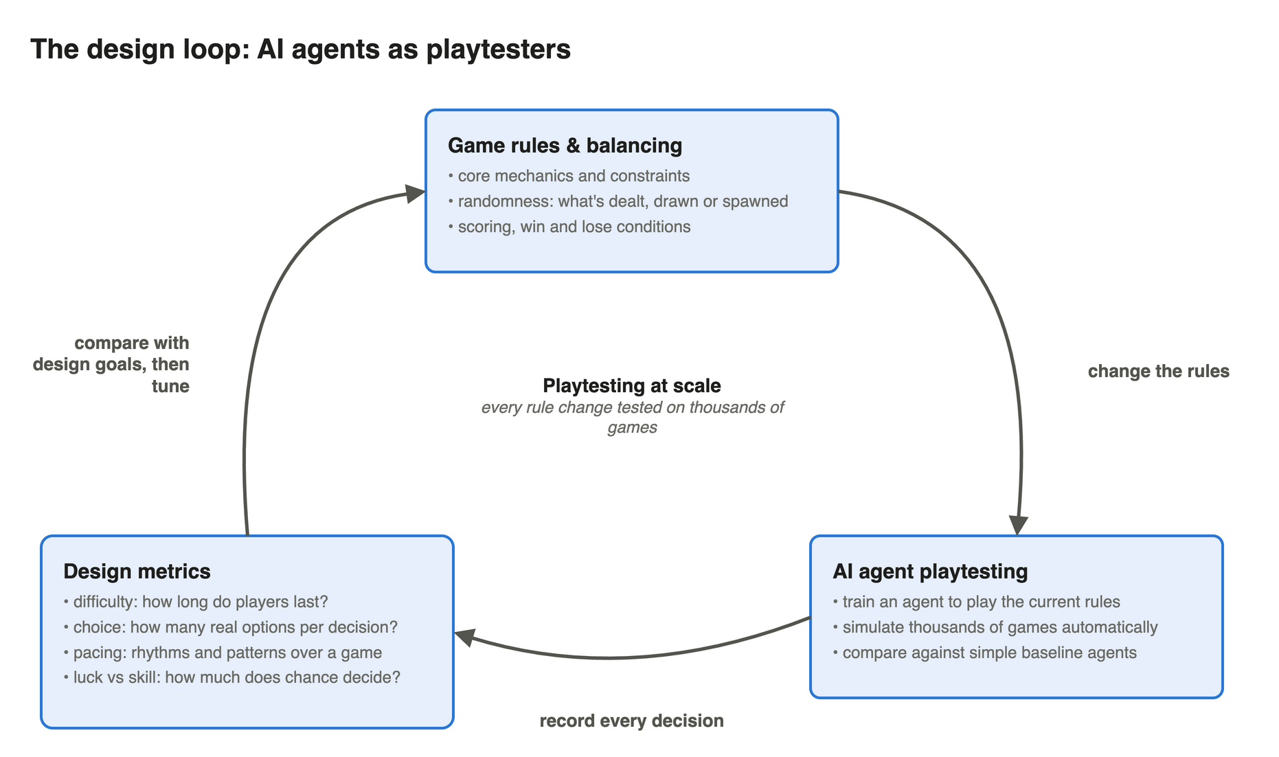
The loop above shows the idea: train an agent to playtest the game, measure design metrics from how it plays, then adjust the rules and balance to hit them. Researchers have been trying this, and variants of it, since at least the late 2000s, and I’ve listed some of the work I’ve found most interesting in Related work at the end.
As an initial step into this world, I’m going to look at AI agent playtesting and design metrics in the already highly successful puzzle game 1010! by Gram Games (available on the App Store and Google Play). I’ll show how we can train an agent to play the game and uncover some of the reasons its game dynamics work so well. If you’ve not played 1010! before, feel free to skip to the results section where you can have a quick play of my version.
Design principles
Let’s now look at two design principles that are interesting to explore in 1010!, and that we can easily build metrics for.
But before we do that, I think there’s an important caveat to point out. Choosing which principles (and metrics) to focus on is part of the creative process. Designers will naturally want to focus on different things, leading to games that are fun in different ways. This isn’t a case of AI taking over and deciding what is/isn’t fun.
Complexity of decision-making
During a typical game is there an overwhelming number of plausible moves that can’t easily be narrowed down to one or two good ones? Or maybe there is a uniform distribution of plausible moves, which makes the player feel it doesn’t matter what they choose. How does this distribution change over time? Does it start with a small number of possibilities and then balloon rapidly as the game evolves, leaving the player feeling overwhelmed?
Inevitability of outcome
Once you’re part-way through a typical game, how inevitable is the survival outcome based on your play so far? e.g. does a mistake on turn 2 massively impact your chance of survival 100 moves later, or does it only impact your survival chances over the next 10 moves? The latter feels much better to players as it makes them feel they still have something to continue to play for even if things aren’t looking great.
Methodology
Here’s the setup. I’ve kept this section fairly light, the full details are in the Appendix for anyone who wants them. All the code, including the game, the training and the analysis, is on GitHub at mattdown/PyTenTen.
The game
I implemented a 1010!-style block puzzle in Python. The rules are:
- A 10×10 grid that starts empty.
- You’re dealt a hand of 3 random pieces. You have to place all 3, in any order, before you get the next 3.
- There are 19 piece shapes, the same set as the real game (a single dot, lines, squares and L shapes), and they can’t be rotated.
- Any completely filled row or column is cleared.
- It’s game over when none of the pieces left in your hand fit anywhere.
For scoring I’ve used turns survived, i.e. the number of pieces placed. The real game awards points for line clears, but survival is what actually matters and it keeps the analysis simple.
The 3-piece hand turns out to be quite important. It means every game runs in exact 3-move cycles, and you’ll see that rhythm show up all over the results.
Game agent
The agent is about as simple as it gets. It’s a small convolutional neural network (CNN) that looks at a position (the board plus the pieces still in hand) and outputs a single number, the value of that position. This is roughly “how many more turns do I expect to survive from here?”.

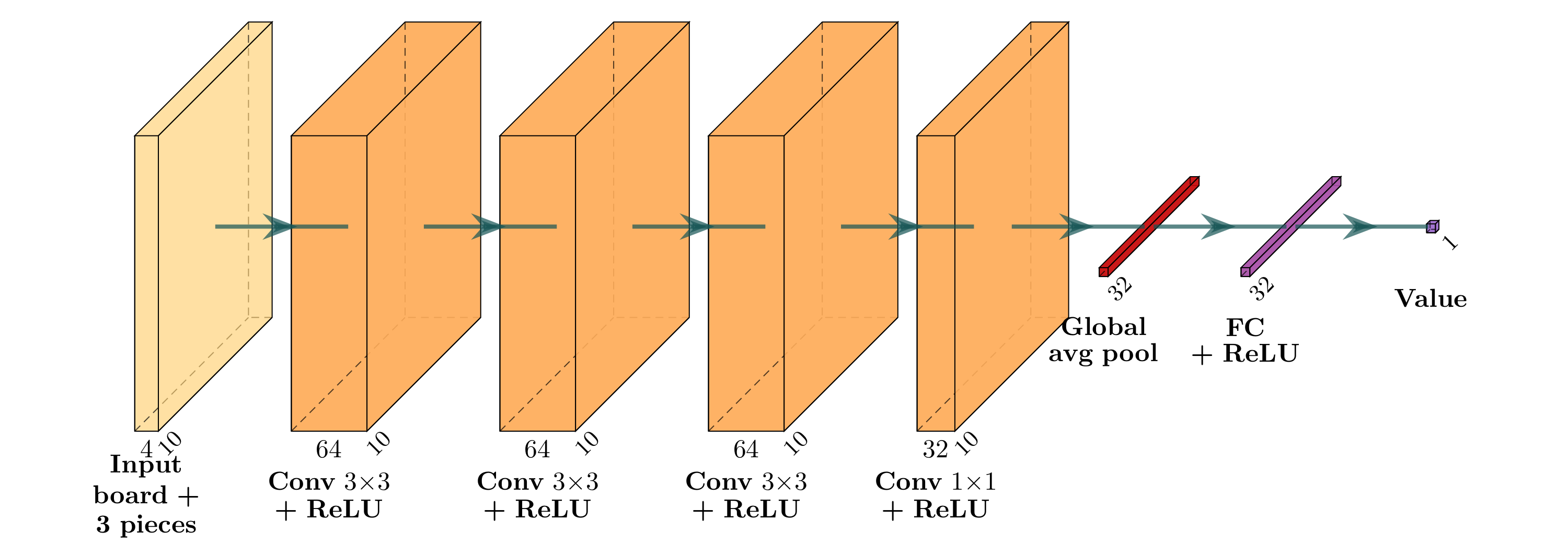
To pick a move, the agent tries every legal placement, asks the network to rate each resulting position and plays the highest-rated one. There’s no look-ahead or tree search, it’s purely greedy. The network is tiny, only ~79k parameters.
For training, a hand-written heuristic agent (which likes clearing lines and dislikes leaving holes) played the first batch of games. The network learned from those, overtook the heuristic after a single round, and from then on learned from its own games (self-play). The whole thing took ~4 hours on a laptop.
Designed to generalise
The network’s shape was a deliberate choice, with the wider design loop in mind. It isn’t tied to 1010!’s exact set of pieces or its 10×10 board, which matters a lot when the end goal is to change the rules.
- Different piece shapes. Each piece in hand is drawn into its own input channel as a picture of the piece (its 5×5 layout), not as an ID from a fixed list of shapes. The convolutional layers then learn local patterns, such as edges, gaps and filled runs, that apply to any shape. A new piece is just a new picture, so it can go straight into the same network without changing its structure.
- Different board sizes. Every convolution keeps the grid size as it is, and the only step that collapses the grid down to a single set of features is the global average pooling at the end. So the same weights accept an 8×8 or a 12×12 board just as happily as a 10×10 one. There’s no layer that only works for 100 cells.
- Any set of moves. The network rates positions rather than outputting one score per possible move, so the action space isn’t baked in either. A bigger board or a new piece simply means the agent tries more placements.
Being able to take these inputs isn’t the same as playing well with them. I haven’t tested this yet, and a variant that’s far from what the network was trained on will likely need some extra training. But starting from a network that already understands the basics should be much cheaper than training a new agent from scratch for every variant. That’s what makes it practical to explore far more of the design space: new piece sets, different board sizes and different piece odds can all be tested with the same agent.
Unity - Python pipeline

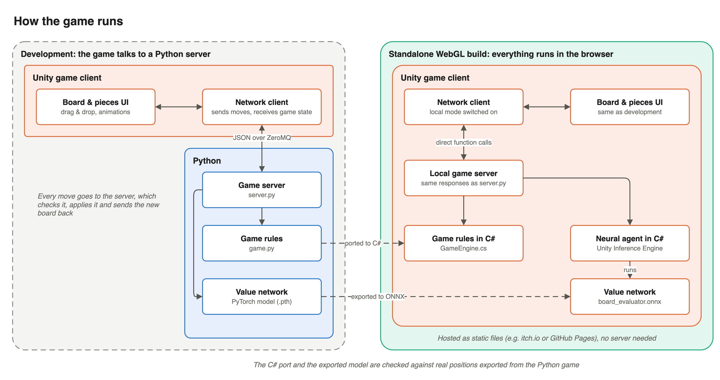
During development, all the game logic lives in Python. The Unity client only handles the board, drag and drop and animations. It sends each move to a Python game server as JSON over ZeroMQ, and the server checks the move, applies it and sends the new board back. That way there’s a single copy of the rules, shared with training and the analysis.
The big advantage of setting it up like this is that the game lives right next to the machine learning code, so the model can be trained directly with PyTorch. Training plays its games in Python without Unity in the loop, so it can get through thousands of them quickly.
The web version you can play below has no Python server to talk to, so the rules were ported to C# and the network exported to ONNX, which runs in the browser with Unity’s Inference Engine. The client has a local mode that gives the same responses as the Python server, so the rest of the game doesn’t know the difference. To make sure nothing got lost in translation, the C# port and the exported model were checked against real positions exported from the Python game.
Calculating and defining metrics
Now to turn the two design principles from earlier into hard metrics that can be measured.
Complexity of decision-making → entropy
The natural tool here is Shannon entropy, measured in bits. If you have $N$ equally good options, the entropy is $\log_2 N$ bits, so it’s easy to turn back into a count: $2^H$ is the “effective number of options”. 4 bits is like choosing between 16 equally good moves, 0 bits means there’s only one sensible move.
I measure two versions of this at every turn:
- Legal-move entropy, $H = \log_2 N$ where $N$ is the number of legal moves. This is how much freedom the board gives you.
- Agent entropy. The network rates every legal move, and I turn those ratings $v_i$ into probabilities with a softmax, then take the entropy:
$$p_i = \frac{e^{v_i/T}}{\sum_j e^{v_j/T}}, \qquad H = -\sum_i p_i \log_2 p_i$$
If many moves are rated about the same, the entropy is high and the decision is genuinely hard. If one move clearly stands out, it’s close to 0. This is the one that maps onto “plausible moves that can’t easily be narrowed down”. Note the agent always plays its top move, the softmax is purely a measuring tool. ($T$ is a temperature setting, see the appendix.)
Inevitability of outcome → does a bad position stay bad?
Here I use the network’s value directly. If the outcome is inevitable, a bad position now should mean a bad position later, and players who fall behind should rarely recover. So I look at:
- Autocorrelation of the value: if a position is rated above average now, is it still above average $n$ moves later? This tells us how long the network’s rating “remembers” anything.
- Dips and recoveries: I call it a dip when the value falls into the bottom 10% of mid-game values, and a recovery when it climbs back to the typical (median) value before game over. What fraction of dips recover, and how quickly?
Results
Here are the results. But first, here’s the Unity game with the agent offering hints to give you an idea of how it plays. Note that the network runs on-device, in the browser, and it’s fast enough that it could also work as a hints system in a production build. This is an unofficial recreation made for research purposes.
All the results below come from 1000 games played by the agent, 911,503 moves in total.
Agent training
Here’s how the trained agent compares with the heuristic and with random play:
| Agent | Games | Mean turns survived | Median | Best |
|---|---|---|---|---|
| Random | 500 | 18.5 | 17 | 38 |
| Heuristic | 500 | 283 | 209 | 1487 |
| Neural network | 1000 | 912 | 634 | 6035 |
So the network survives ~3.2× longer than the heuristic and ~49× longer than random play. That’s pretty good for a network this small with no look-ahead.

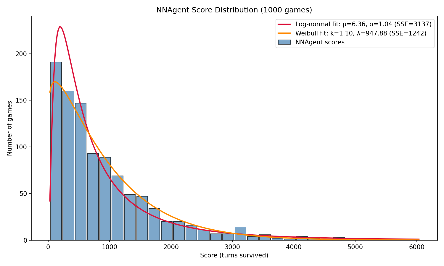
The spread of scores is interesting in its own right. It’s heavily skewed: most games end within a few hundred turns, but there’s a long tail running past 3000. The best fit, by a clear margin, is a Weibull distribution with a shape close to 1 (k = 1.10), which means an almost constant risk of dying on every move, however long the game has lasted. Every new hand is a fresh roll of the dice, another chance to be dealt something that doesn’t fit. Keep that in mind, luck comes back later.
Complexity of decision-making

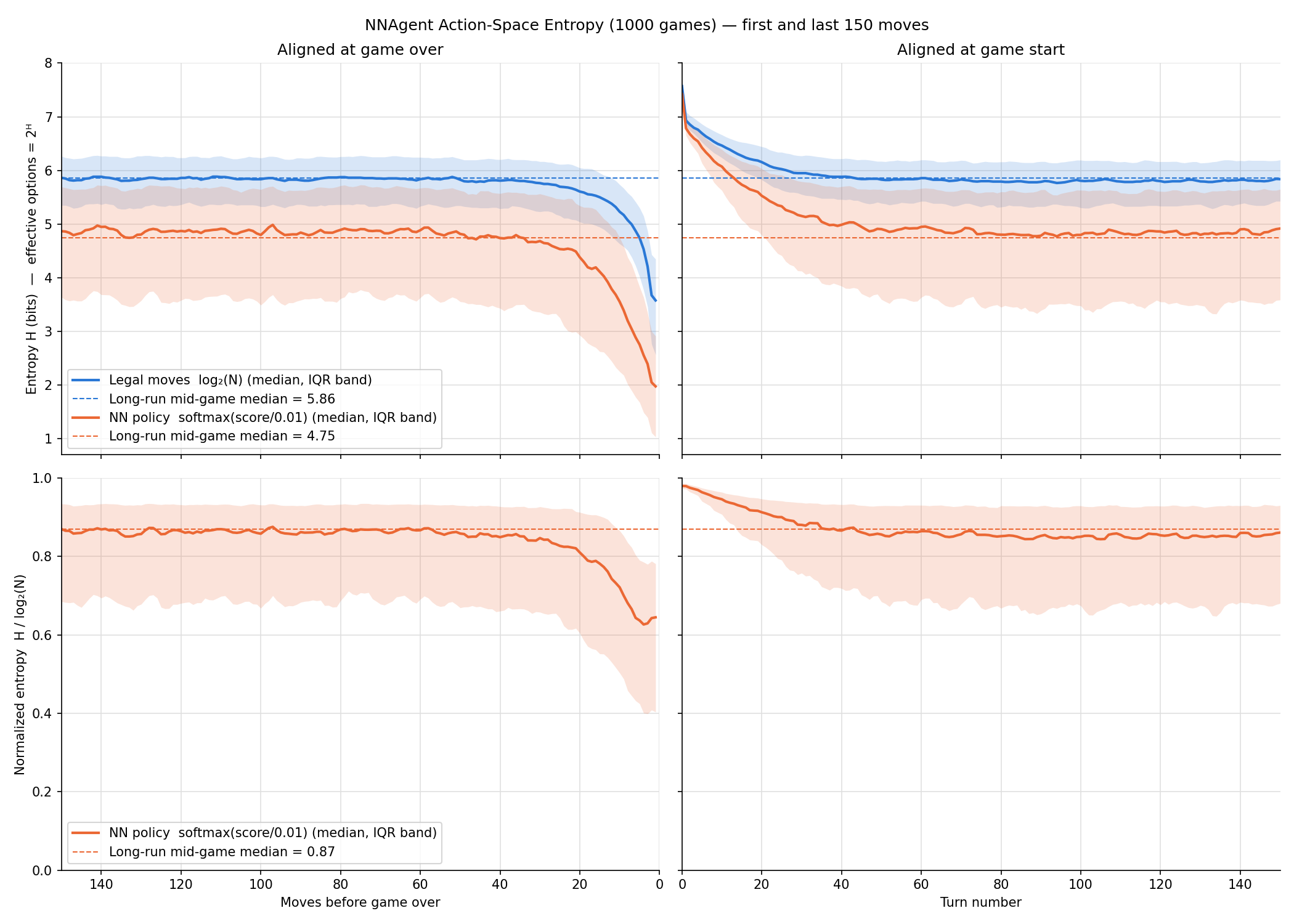
The top row shows both entropies at the start and end of a game (blue for legal moves, orange for the agent). I’ve cropped it to the first and last 150 moves, because that’s where everything happens. The middle of the game is flat all the way through. On the left the games are lined up by when they ended, on the right by when they started. Lines are the median across games, the bands cover the middle 50%, and the dashed lines are the typical mid-game value.
A few things stand out:
- There’s a lot of choice, but it can be narrowed down. A typical mid-game board allows ~58 legal moves (5.9 bits), but the agent only treats ~27 of them as serious candidates (4.75 bits). That feels like a good place for a puzzle game to sit. It’s far from obvious, but it’s not an overwhelming Go-style wall of options either. And it’s not the case that every move is as good as any other.
- It’s remarkably flat. After the opening (the empty board allows loads of moves), the legal-move count settles within ~40 turns and the agent within ~50. Then both sit on the dashed line for hundreds, even thousands, of moves. The board doesn’t slowly fill up over time.
- Then it collapses. The agent’s entropy starts to fall ~35–40 moves before game over, about 10 moves before the legal-move count, and both drop steeply over the last ~10. That fits running out of good moves before you run out of legal ones.
- The agent gets more decisive under pressure. The bottom row divides the agent’s entropy by the legal-move entropy. It starts near 1 on the empty board (almost every move looks fine), settles at ~0.87, then drops to ~0.63 over the last ~25 moves as one move increasingly stands out.
The medians hide a lot of move-to-move variety though. Here are the first 100 moves of 10 individual games, with each hand of 3 shaded:

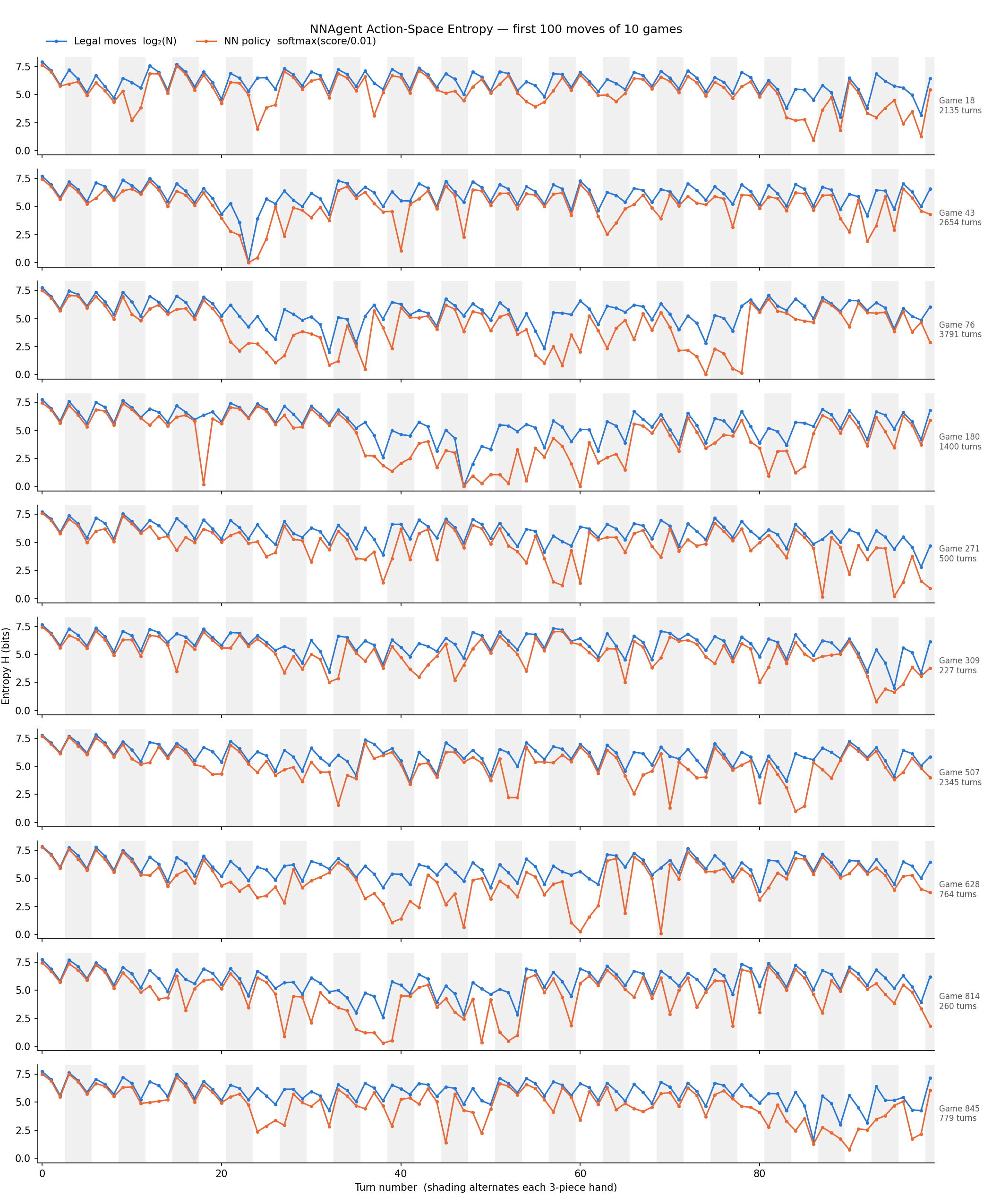
The legal moves (blue) follow a very regular sawtooth: the most freedom on the first piece of each hand, the least on the last. The agent (orange) is more interesting. There are one-off spikes down to ~0 bits where one move is clearly best (probably a line clear on offer), and longer troughs lasting several hands when the board gets tight, e.g. game 180 around turns 35–62 and game 814 around turns 33–53.

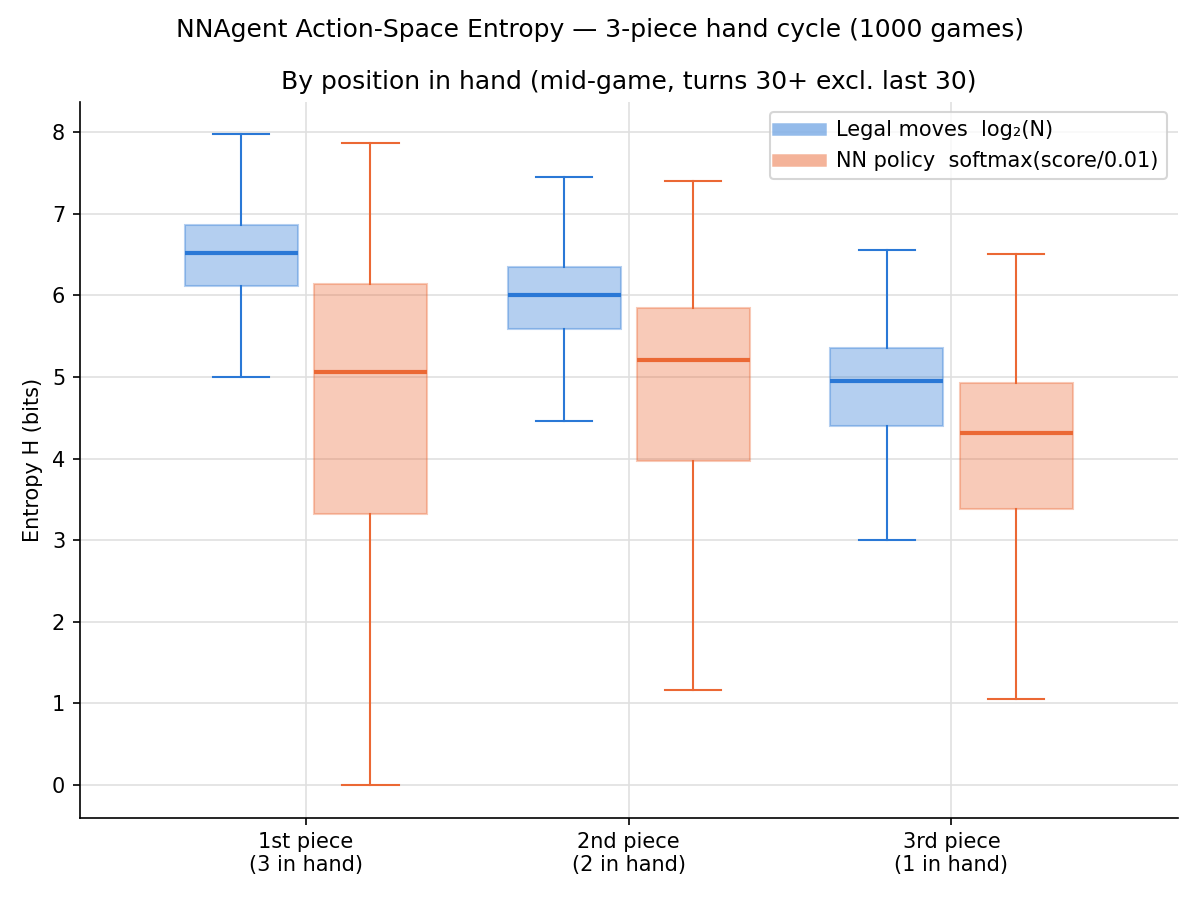
Splitting the mid-game up by position in the hand makes the rhythm clear. The boxes cover the middle 50% of moves, and the medians are:
| 1st piece (3 in hand) | 2nd piece (2 in hand) | 3rd piece (1 in hand) | |
|---|---|---|---|
| Legal moves | 6.52 bits | 6.00 bits | 4.95 bits |
| Agent | 5.06 bits | 5.21 bits | 4.31 bits |
The legal moves fall by ~1.6 bits across every hand, from ~90 options on the 1st piece to ~30 on the 3rd. With one piece left there’s nothing easier to fall back on, so the last piece is where the board runs out of room.
The agent’s cycle is much weaker. The 3rd piece is the most decisive, but the 2nd is actually the hardest call, not the 1st. More telling is the size of the agent’s boxes: they’re far taller than the legal-move ones and overlap heavily, so how hard a decision is depends much more on the position than on where you are in the hand. My guess (untested) for the 1st piece is that with 3 pieces the playing order matters a lot, e.g. setting up a line clear, which makes one move stand out.
Inevitability of outcome

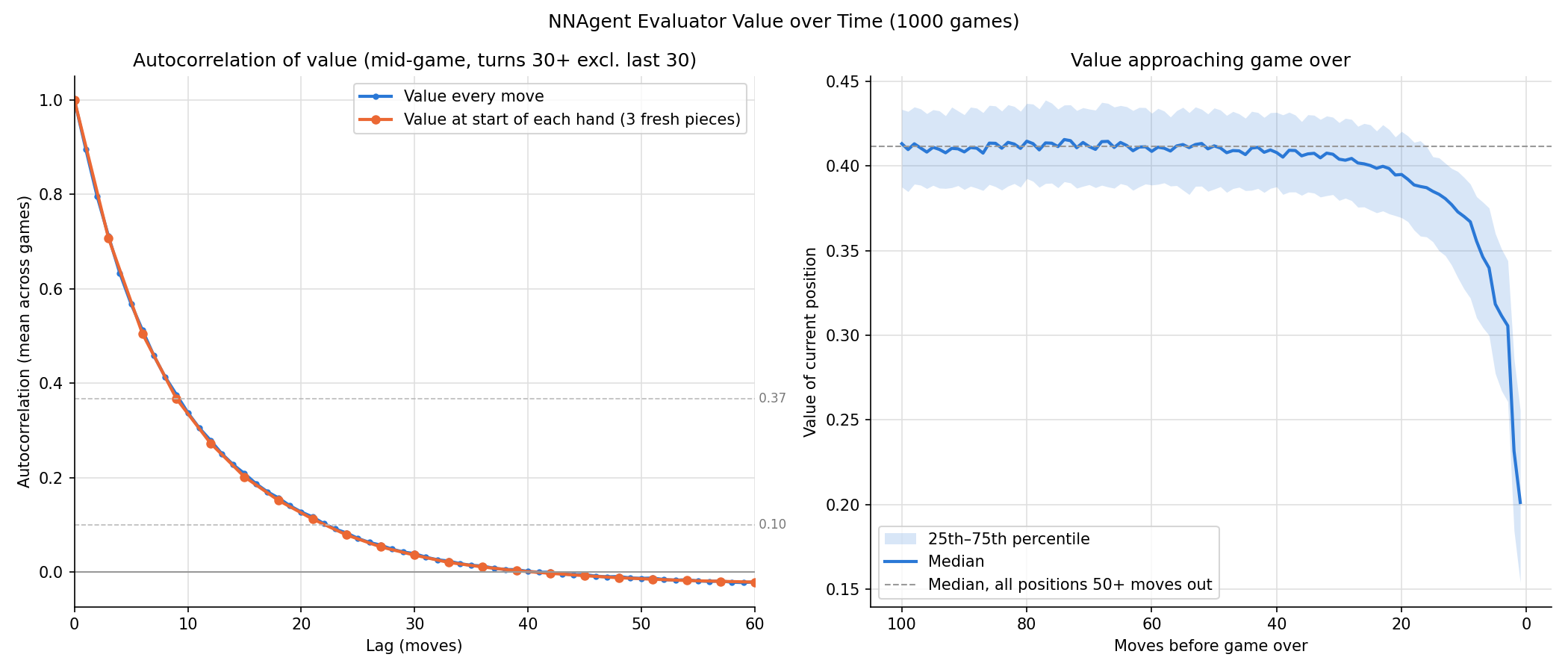
The left panel is the autocorrelation of the network’s value. It drops below 1/e (a common “it’s mostly forgotten” threshold) after 10 moves, and is essentially gone by ~23 moves. In other words, knowing a position is good or bad right now tells you very little about how things will look 6 hands later.
The right panel shows the median value in the run-up to game over. It’s flat until ~20–30 moves before the end and only then starts to fall. The network rates a game with 50 moves left the same as one with 500. As far as the network can tell, beyond ~20 moves the outcome comes down to pieces that haven’t been dealt yet.
Now for my favourite chart:

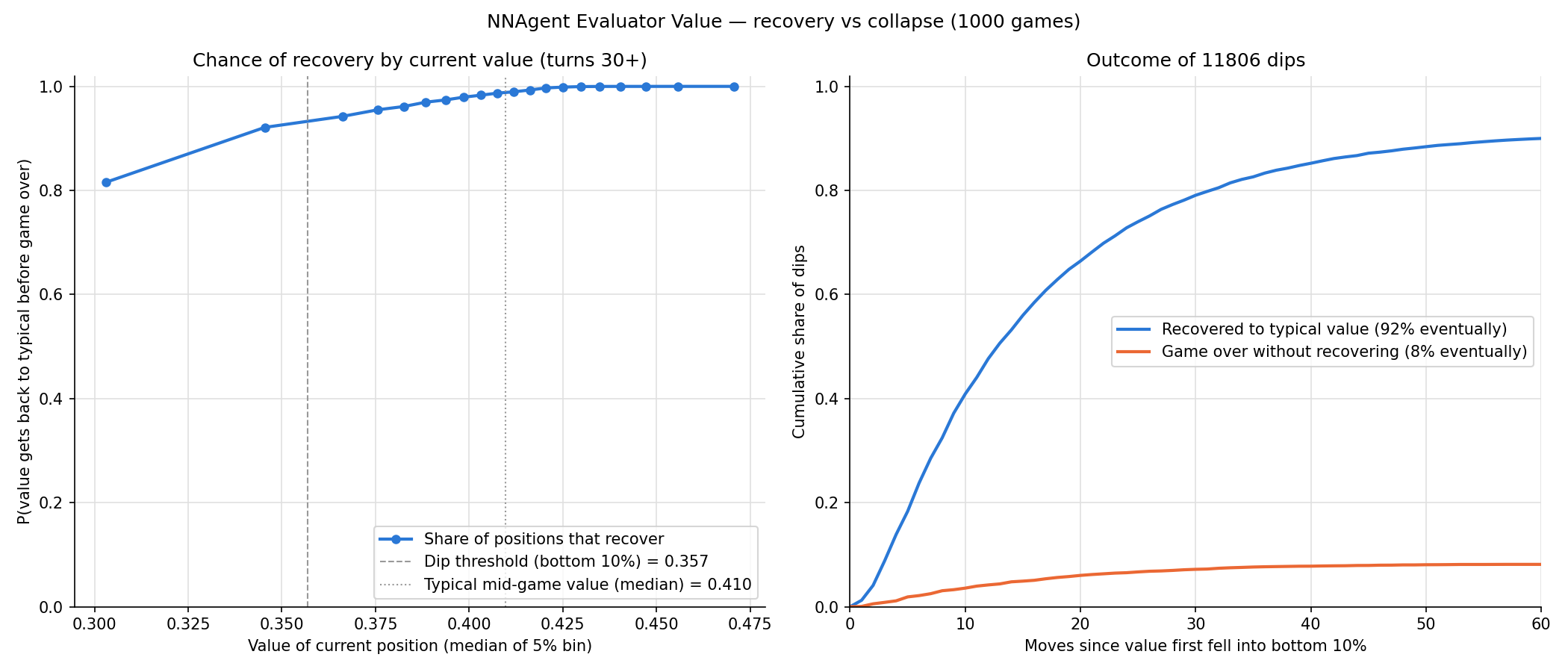
On the left is the chance that a position gets back to a typical value before game over, plotted against how bad it is right now. On the right, for all 11,806 dips across the 1000 games, is the share that have recovered (blue) or hit game over (orange) as the moves go by.
- 92% of dips recover, with a median of 12 moves.
- 8% end in game over, also with a median of 12 moves.
- Almost every dip is settled one way or the other within ~35 moves.
- There’s no point of no return. The chance of recovery falls smoothly as the position gets worse, and even the worst 1% of positions recover 64% of the time.
So you can usually get out of a bad position quickly, unless you can’t, and then it’s over just as fast.
You can see this in individual games too. Here are the last 100 moves of the same 10 games as before, with the typical value (dashed) and the dip threshold (dotted):

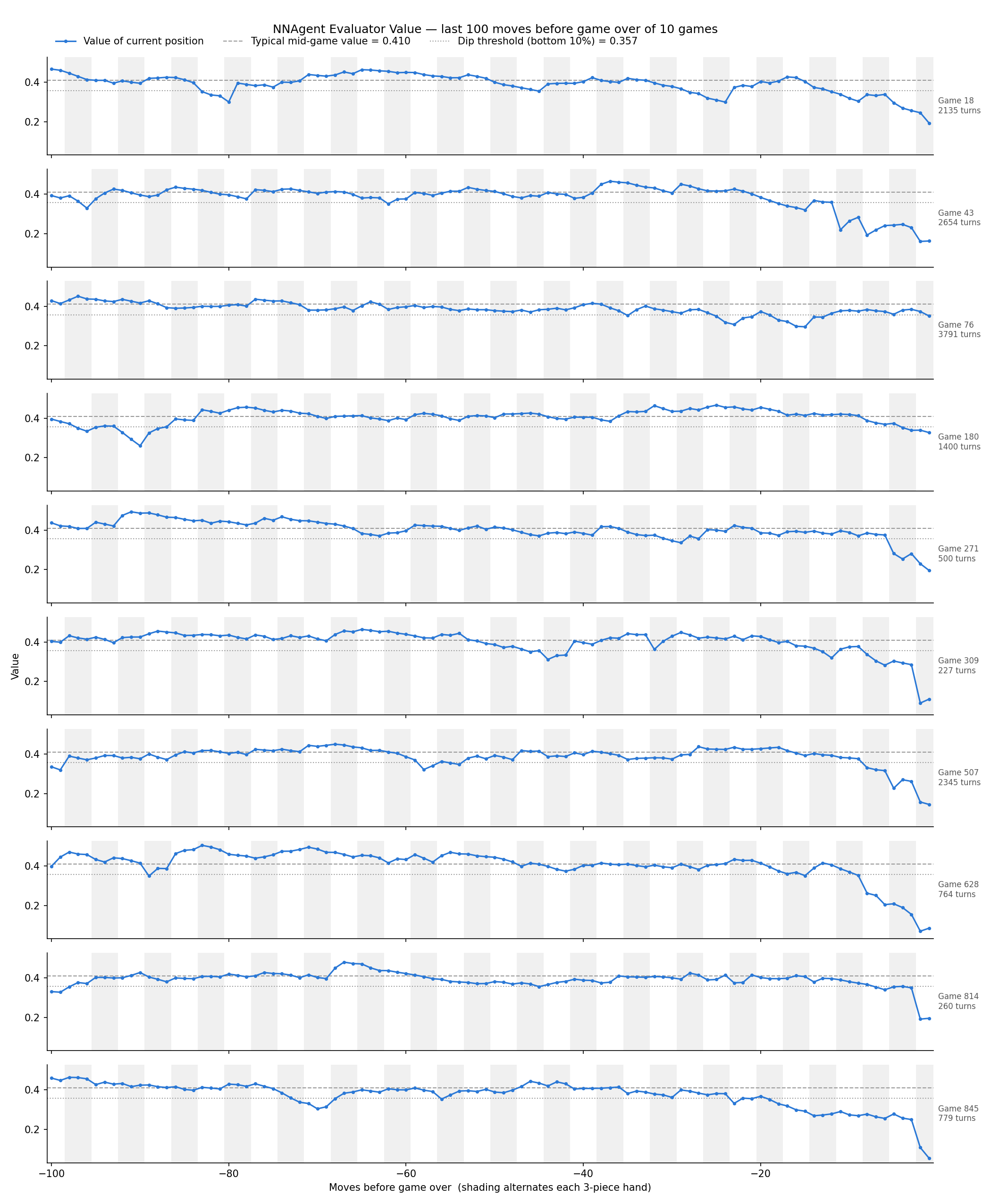
The endings come in roughly three flavours:
- A steady slide over the last ~20–30 moves (games 18 and 845), or a faster one over the last ~10 (game 628).
- Sudden death. Game 814 sits near the dip threshold until the last 2 moves, then drops. Game 309 falls off a cliff in the last 2 moves, and game 271 in the last ~5.
- Barely any warning at all. Games 76 and 180 are only around the dip threshold when they die.
What do these metrics tell us about 1010!?
On complexity of decision-making, 1010! sits in a sweet spot. There are always plenty of legal moves, but the agent can narrow them down to a manageable shortlist of ~27. That stays consistent for the whole game, until the final crunch.
On inevitability of outcome, 1010! is very much not inevitable, and I think that’s a big part of why it works. Being halfway through a game tells you almost nothing about how it’ll end. A bad position is usually recoverable, and even a really bad one gives you a fighting chance. But recovery isn’t guaranteed either, so there’s always some tension. As a caveat, all of this is measured through the network’s opinion, which has its own blind spots (more on this in the appendix).
When designing new casual puzzle games these can be used to guide your own game dynamics, both in terms of the design principles, but also the exact numbers that 1010! hits.
That’s only half of the loop from the intro, and it’s as far as I’m going to take 1010! for now. Rather than rebalancing a game that already works, the real power of this approach is in designing new games from scratch, and that’s what I’ll look at next.
Related work
Using AI players to explore game designs has a surprisingly long history. Here’s some of the work closest to this post, if you want to dig deeper:
- Measuring what makes a game good. Cameron Browne’s Ludi system (Evolutionary Game Design) evolved new board games and scored them through self-play against 57 aesthetic criteria. These include drama (players should have hope of recovering from bad positions) and uncertainty (the outcome should remain uncertain for as long as possible), which are very close to the inevitability metric here. One of its games, Yavalath, became the first commercially released board game designed entirely by a machine.
- Exploring a game’s parameter space. Isaksen, Gopstein and Nealen’s Exploring Game Space Using Survival Analysis used an AI player to explore thousands of variants of Flappy Bird, predicting each one’s difficulty from the distribution of scores.
- Changing the rules with a superhuman agent. DeepMind’s Assessing Game Balance with AlphaZero, with former world champion Vladimir Kramnik, trained AlphaZero on nine rule variants of chess and compared how decisive each one was. This is the full design loop from the intro, just with a vastly bigger agent.
- Mobile puzzle games. Roohi et al.’s Predicting Game Difficulty and Churn Without Players combined deep reinforcement learning agents with a simulated player population to predict pass rates and churn for each level of Angry Birds Dream Blast.
- Letting AI change the rules too. More recently, language models have started to take on the designer’s side of the loop. GAVEL uses a language model to mutate and recombine board games written as code, and RuleSmith uses LLM agents playing each other, plus Bayesian optimisation, to tune the rules of a civilization-style game for balance.
Appendix
A. Game details
- Pieces: the 19 shapes of the real 1010!, drawn uniformly at random with no rotation (the real game’s piece
odds aren’t public, so uniform is a stand-in):
- a single 1×1 dot;
- lines of 2, 3, 4 and 5 cells, horizontal and vertical (8 shapes);
- 2×2 and 3×3 squares;
- small (3-cell) and large (5-cell) L shapes, 4 rotations each.
- Clearing: several rows and columns can clear at once.
- Reward: +1 per move survived. Points for line clears exist in the code but are switched off.
- Turn limit (training only): while generating training data, games are stopped at 2000 turns so a strong agent can’t play forever. The results and the comparison table have no limit: every game is played to game over.
- Action space: 3 pieces × 14 × 14 anchor positions = 588 possible actions, most of which are illegal at any given moment. The anchor is the top-left of the piece’s 5×5 bounding box, from −4 to 9 on each axis.
B. The agents
| Agent | How it picks a move |
|---|---|
| Random | A uniformly random legal move. |
| Heuristic | Tries every legal move and scores the result: +1000 per line cleared, −10 per hole (an empty cell boxed in on all 4 sides), −1 per edge between filled and empty cells (roughness). |
| Neural network | Tries every legal move and asks the network to rate each resulting position (board + remaining pieces). Plays the highest-rated one. |
C. Network architecture
- Input: 4 channels on a 10×10 grid.
- Channel 0: the board (1 = filled).
- Channels 1–3: one per piece in hand, with its 5×5 layout in the top-left corner and the rest zero. A piece that has already been played is all zeros.
- Trunk: 3× Conv 3×3 (64 channels, padding 1) + ReLU. There’s no pooling, so the 10×10 grid is kept the whole way through.
- Value head: Conv 1×1 (32 channels) + ReLU → global average pooling → fully connected 32 + ReLU → fully connected 1.
- Size: 79,393 parameters.
What the value means. The network is trained to predict the discounted number of future turns survived, $\sum_k 0.98^k$ over the remaining moves, scaled to [0, 1]. A discount of 0.98 gives an effective horizon of ~50 moves, so positions 100 or 500 moves from death have almost the same target. The network is never asked to tell them apart.
What it’s shown. The network is trained on after-states: the board just after a move (lines already cleared) plus the pieces still waiting. That’s exactly what the agent asks it to rate when choosing a move. After the last piece of a hand, the after-state has an empty hand, because the next hand hasn’t been dealt yet, so the network learns the value averaged over whatever hand comes next. The “value of a position” in the charts is the network’s score for the best move available there.
D. Training

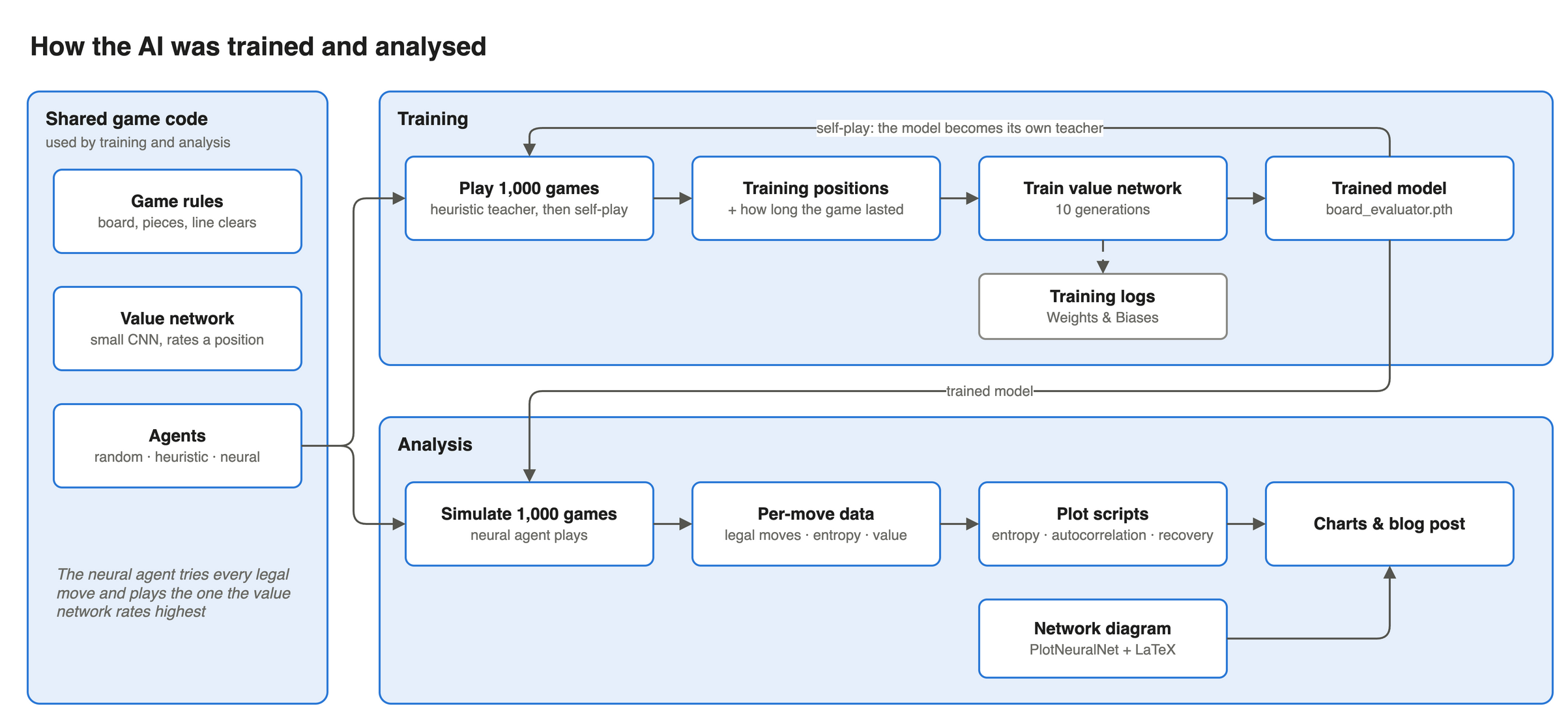
- Data generation: each generation plays 1000 games with a “teacher” agent, which makes a random move 50% of the time for variety. Every after-state is recorded with its discounted return, computed backwards from game over (+1 per move, discount 0.98). The targets are scaled by the largest return seen. Games are stopped at 2000 turns, and in a stopped game the last 200 positions are dropped, because their returns are cut short.
- Augmentation: each position is also added in all 8 rotations and reflections. The board and the pieces are transformed together, so the pieces still fit.
- Optimisation: mean squared error, Adam (learning rate 0.01, weight decay 1e-4), batch size 8000, 20 epochs per generation. The learning rate is halved when validation loss stalls (patience 3), with an 80/20 train/validation split. The best validation checkpoint within each generation is kept.
- Curriculum: the heuristic is the teacher at first. Once the network out-survives the heuristic by 5% (over 50 games each), it switches to self-play. 10 generations in total.
- How it went: before training the network survived 23 turns, against the heuristic’s 245. After generation 1 (heuristic data only) it survived 746, beat the heuristic and switched to self-play. Self-play generations take ~35 minutes each, because the games are long. The run was done in two parts: the first stopped partway through generation 6, and the second resumed from the best generation-6 checkpoint for the remaining 4 generations. That’s ~4 hours in all on an Apple Silicon GPU. The final model is the best checkpoint of the last generation (validation loss 0.0268). Survival kept improving, from ~650 average turns at generation 6 to 912 at generation 9.
E. Metric details
- Temperature. All agent-entropy charts use $T = 0.01$. The network’s scores are in [0, 1] and the gap between the best and the median move is only ~0.01–0.06, so at $T = 1$ every move would look equally likely. $T$ is a free parameter. The patterns hold across temperatures, but the absolute numbers depend on it.
- Normalised entropy: $H / \log_2 N$, from 0 to 1. This is the agent’s decisiveness relative to how many options it has (the bottom row of the entropy chart). It sits at ~0.87 for most of the game and dips to ~0.63 at the end.
- Mid-game: turn 30 onwards, excluding the last 30 moves. Used for the steady-state analyses, because entropy and value are still settling after the empty board early on, and collapse at the end.
- Autocorrelation at lag $n$: the correlation between a quantity at turn $t$ and at turn $t + n$, using each game’s differences from its own mid-game average, averaged across games (only games long enough for the lags shown).
- Hand cycle removed: before correlating, subtract each game’s average for each position in the hand (1st, 2nd, 3rd piece). This leaves only structure slower than the 3-move rhythm.
- Dips: the typical value is the median mid-game value, 0.410. A dip starts when the value first falls into the bottom 10% of mid-game values (below 0.357), and a new dip can only start after the previous one has recovered. 978 of the 1000 games ended in a dip that never recovered. The other ~2% died without ever reaching the bottom 10%, a sudden death from a bad deal.
F. Extra charts
Entropy autocorrelation. The same autocorrelation idea applied to entropy, raw (left) and with the hand cycle removed (right):

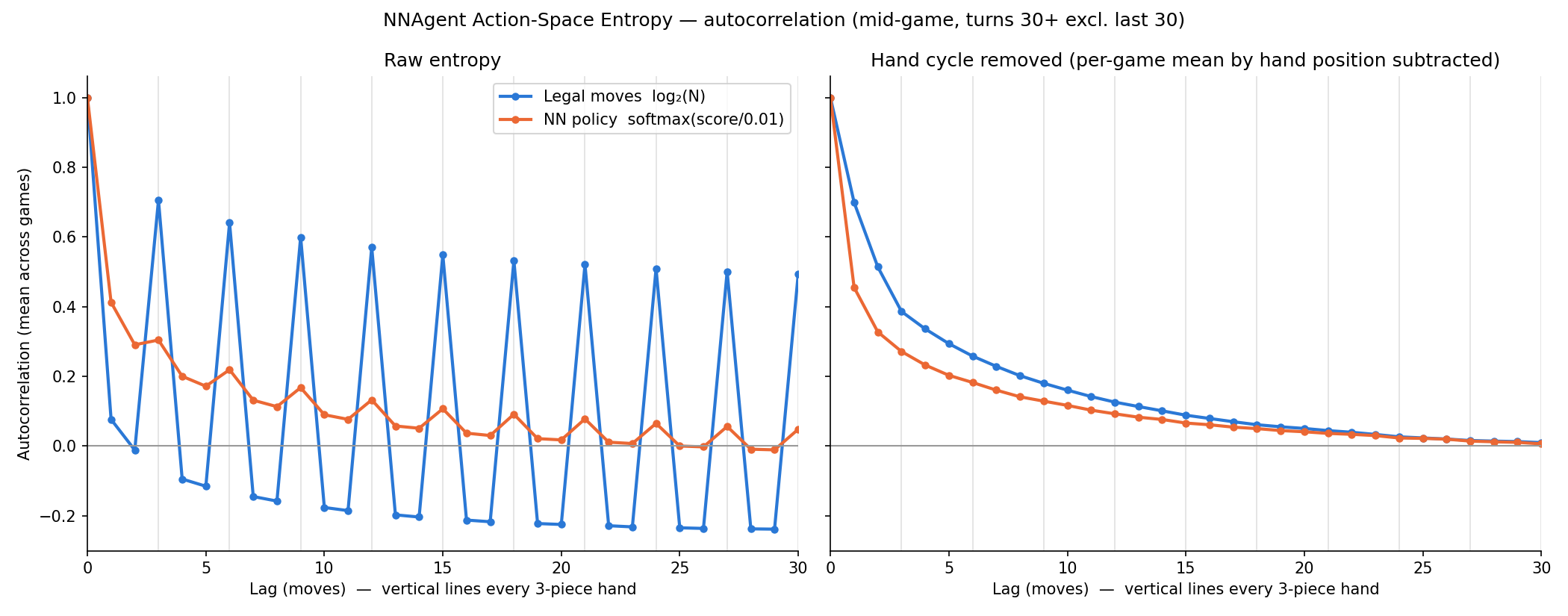
The legal-move entropy has sharp peaks every 3 moves that barely fade, because the game deals a new hand every 3 moves regardless. With the cycle removed, it decays smoothly to ~0 by ~20 moves and never goes negative, so there’s no longer hidden cycle, just persistence. A tight board stays tight for a couple of hands, then drifts back. The agent’s entropy decorrelates faster over the first few moves, then follows the same slow tail: its decisiveness is partly move-to-move, with a slower component driven by how tight the board is.
Value in the opening. The first 100 moves of the same 10 games:

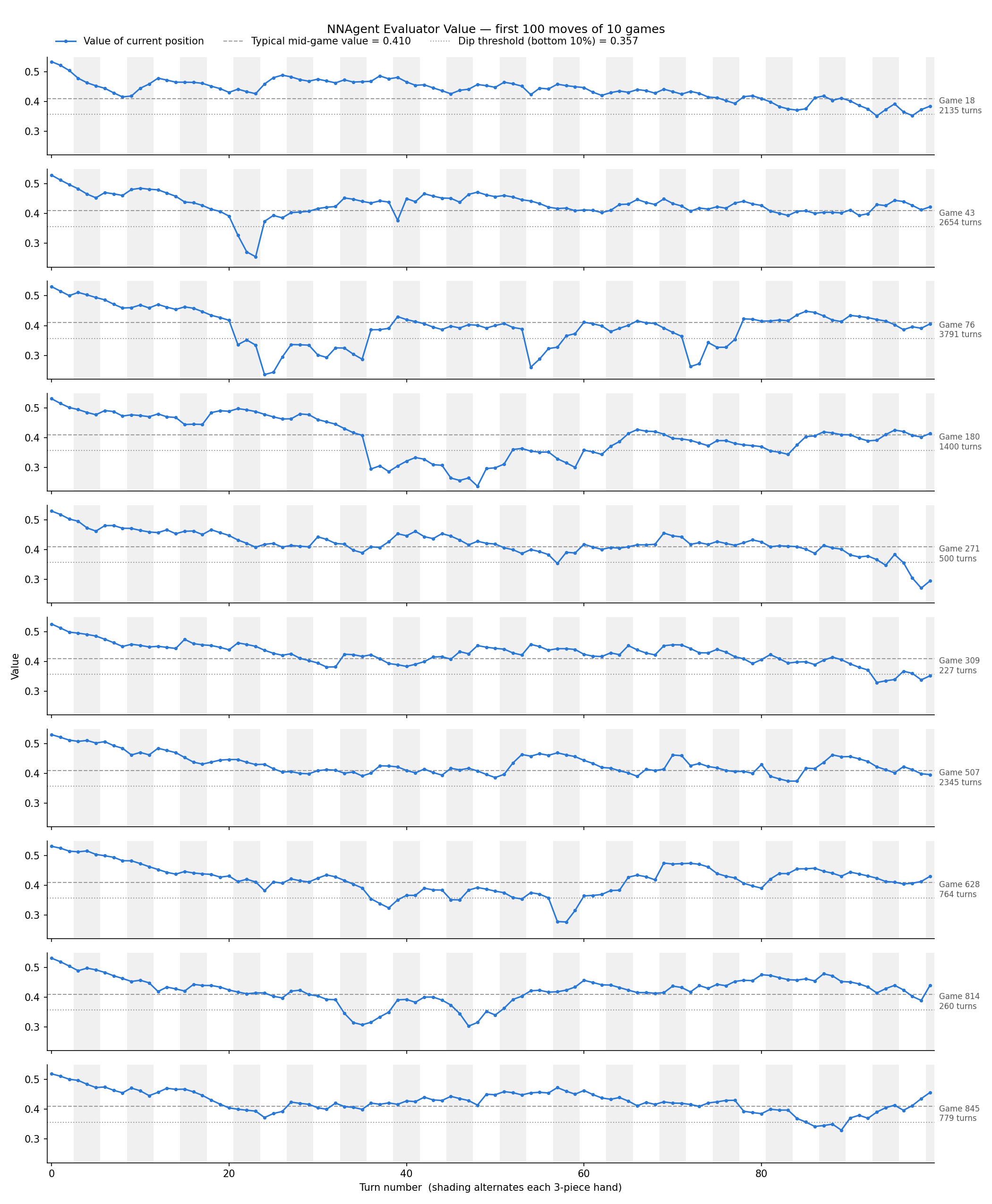
The value starts at ~0.53 on the empty board and settles within ~30 turns. Game 76 has three deep dips in its first 80 moves, each matching an entropy trough, recovers from all of them and goes on to last 3791 turns. Game 180 drops sharply at turn 36 and stays below the dip threshold until ~turn 60, the same stretch as its entropy trough, then recovers. Game 43 has a short, sharp dip around turn 22, when it was down to almost a single legal move, and is back around typical within ~5 moves.
G. Limitations and next steps
- The value is the network’s opinion, not the truth. How short-sighted it is partly reflects how it was trained: a 0.98 discount (a ~50-move horizon) and targets taken from games with 50% random moves, not from its own greedy play. So “how inevitable the outcome is” is measured through the network. A more direct test is to replay the same position many times with different deals and measure how widely the outcomes spread. That’s a good experiment for future work.
- Training games are capped, the results aren’t. The training data stops games at 2000 turns, but ~10% of the games analysed here go past 2000 (the longest lasted 6035). Those late positions look like ordinary mid-game positions, so this probably doesn’t matter much.
- Train for longer. The agent was still improving between generations 6 and 9, so more self-play might make it stronger still.
AI disclaimer: AI tools were used to help with the coding, to build the demo and to write this blog post. The ideas and questions being investigated are my own.