Interactive Monte Carlo Tree Search Demo
Intro
Monte Carlo Tree Search (MCTS) is the famous tree-search planning algorithm used in Google DeepMind’s AlphaGo as well as many other applications. The algorithm itself is relatively simple and should be seen maybe more as a planning algorithm than a learning one.
At a high level, how does MCTS work? Instead of exhaustively searching all possibilities, MCTS searches the state tree in a principled way that prioritises exploration of the most promising paths within that tree.
I always believe the best way to learn is by doing, so check out the demo below. Play on the board in the top right and see how the predicted winner changes as the game progresses. The tree evolves to show which paths work out best for which player. The circle with the highlight indicates the best move. Be sure to zoom in/out to see the full details lower down the tree.
Demo
Algorithm breakdown
Now that you’ve had a play of the demo, let’s talk about how MCTS works. The algorithm starts with just a single node in its tree, but it’s probably easiest to start explaining this algorithm once it’s a few iterations in, so note that the first few iterations will look slightly different to this.
1. Selection
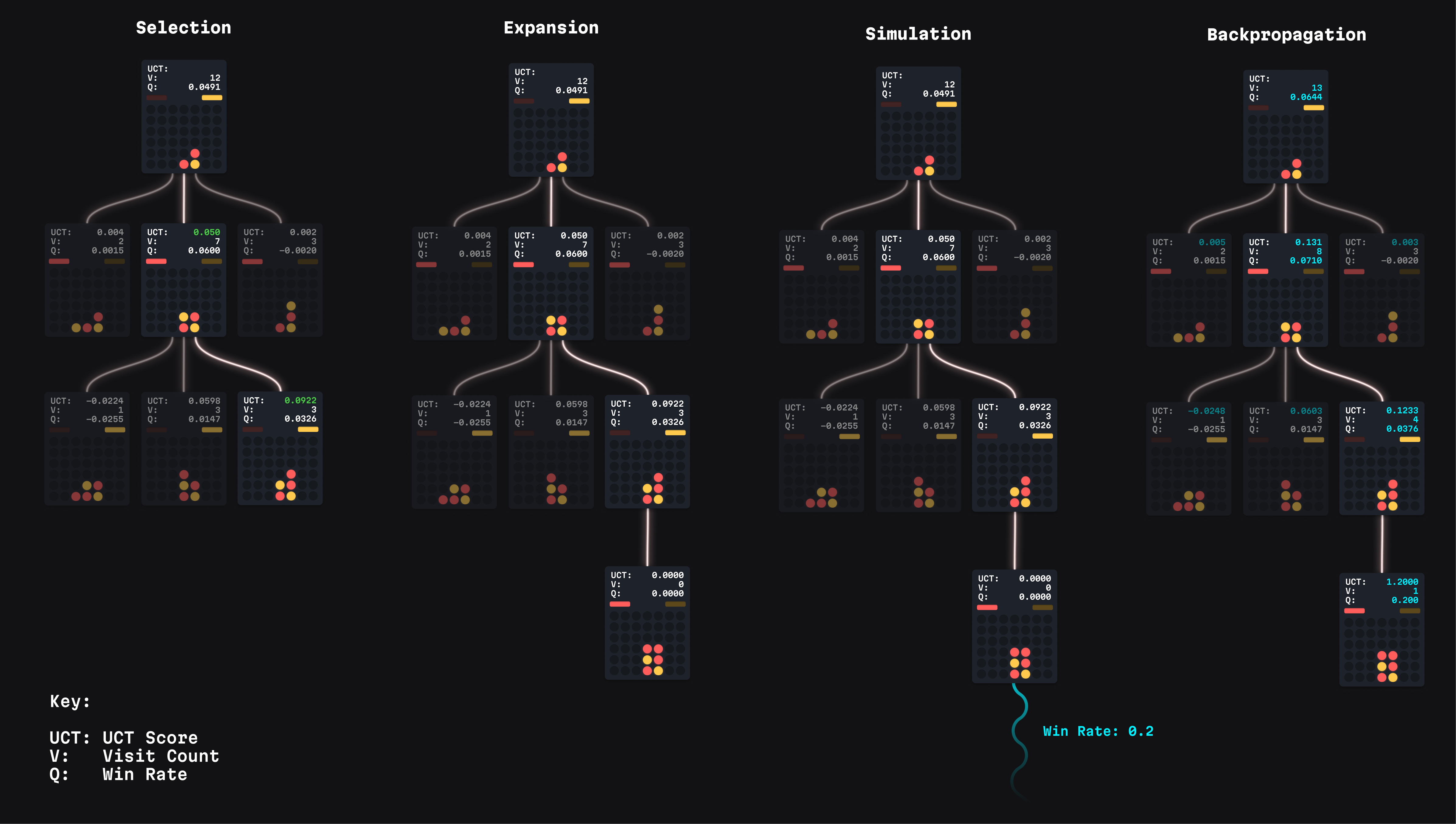
We start at the root node (the current board state) we traverse the tree selecting the maximum UCT score at each node. We’ll explain UCT in a bit, but for now just treat it as a score for the most promising child node.
2. Expansion
When we get to a node with any unexplored children, these unexplored children have an infinite UCT score by definition (as we’ll see below), so one selected at random (if more than one) and added to the tree. In some respects this isn’t really a distinct step as we’re just following the rule above – the only difference is that we’re just considering nodes that exist implicitly rather than actually tracked in memory.
3. Rollout/Simulation
We now do a rollout/simulation from this new node. This consists of playing a simulated game from this node to completion using fast, random moves. In the diagram below, this real-time random probe is represented by the fluid, wavy rollout thread, giving the engine an instant, empirical snapshot of who is likely to win from that state.
4. Backpropagation
Once this simulation is complete, the result (which will be something like a 0.8 win rate for red) is propagated back up the tree, along with incrementing each node’s visit count by 1.
MCTS Diagram
Here’s a diagram representing the above steps:

UCT score
Now let’s take a deeper look at the UCT score (Upper Confidence bound 1 applied to Trees), given by the following formula:
$$UCT = \frac{WinCount}{VisitCount} + C\sqrt{\frac{\log{(VisitCount_{parent})}}{VisitCount}}$$
Exploitation (Left Term): The current calculated value ($Q$). It pulls the AI toward pathways that have already proven successful.
Exploration (Right Term): The uncertainty bonus. It dynamically expands as a parent node gains visits, systematically pulling the AI to investigate neglected sibling options.
Let’s explore these terms further:
The first term is the win rate for this node. A higher win rate suggests a better node/action. This is also referred to as the estimated value of this node and is displayed as Q in-game. $WinCount$ comes from the result of the rollout/simulation and is relative to whoever’s turn it is. During backpropagation the result of the rollout is flipped at each node as it’s added to the $WinCount$ to reflect this. For a single-player game, this wouldn’t be needed.
The second term is inversely related to the number of times this node has been visited relative to its sibling nodes, i.e. low visit counts relative to its siblings will give a higher score. The term in the numerator here $VisitCount_{parent}$ can initially appear confusing as it’s referring to the parent node and not the sibling nodes. Because of the backpropagation step the parent visit count is equal to the sum of the child visit counts and saves us having to sum these each time. The node’s visit count is displayed as V in-game.
The purpose of this second term is to balance exploitation vs exploration. If we only used the value term here we might get a situation where one child node has a win rate of, say, 0.6 with only one visit and a sibling node has a win rate of 0.61 after many visits. It stands to reason that the node with only one visit that has only a marginally lower value score warrants further exploration. The constant $C$ determines the level of exploration and is typically set to around $1.4$
Action selection
Once the tree has been expanded up to a given threshold (number of nodes added) it’s time for the agent to select the best action. Here the UCT score is not used. Instead, the child with the highest visit count is selected. This is because the exploration term in UCT is no longer needed, no time to explore - time to take action now. But simply taking the action with the highest win rate isn’t desirable either as this might select a node with a high value score but low visit count. Total visit count is a better proxy for the child node with the highest true value.
Final remarks
Feel free to check out the demo again now that we’ve gone over the algorithm in more detail. The color of each line/node indicates the value component of the UCT score (win-rate) and the size of the circle indicate the visit count relative to its siblings. These are the parameters used: rollout/simulation count: $5$, expansion count: $10000$ C: $1.4$ but you can change them in the settings menu. Even running on relatively low-end hardware the algorithm plays a mean (but not unbeatable) game of Connect 4 in realtime. Well done if you manage to beat it without the hints. Be sure to flip the ‘Show UCT Score’ toggle in the settings menu to watch the raw UCT, Visit, and Value metrics update across every single node in real-time as the tree expands.
As a final note as to how AlphaGo/AlphaZero uses MCTS – instead of exclusively relying on random rollouts to assess the value of a given node and UCT to select which child nodes to explore. AlphaGo/AlphaZero use MCTS in combination with deep neural networks. One network to act as a value network (better than random rollouts) and another as a policy network (better than a simple UCT score). As you can imagine, the random rollout for moves early in a 19x19 game of Go will be particularly poor at predicting a winner, hence the need for deep neural networks.
I hope you’ve enjoyed this demo. For an extensive review of MCTS and its variants, I recommend this paper: https://arxiv.org/pdf/2103.04931
Finally, if you came here for the Connect 4 there’s actually a better way of solving the game using alpha-beta pruning as explained here: https://www.youtube.com/watch?v=DV5d31z1xTI. I chose Connect 4 for the demo above as it has a limited action space which makes the tree slightly easier to view.